One of the first steps to wrangling network data is to understand how it is structured. This section will walk you through the what network data look like and how it is stored. Then, demonstrate how to bring them into the R environment. Finally, we will work on converting these data objects into network objects in R using the igraph package.
LEARNING ELEMENTS - Data Perspectives
Consider that social network data can be sensitive! It is ethical to de-identify people in the networks. We deal with fictional characters or public figures with pseudonyms in these exercises.
Network data are notoriously difficult! An important aspect of any research is to recognise the limitations of your data. Your network may not be representative of the whole group you are studying (let’s say not everyone is represented in the network). So, you need to either seek more representative data, or simply admit these limitations in whatever report or article you are writing.
Keep in mind, you will be using network data that is already stored into (relatively) clean formats. Outside of this book, you may be working with data that are not so cleanly identifiable as network data. For example, you may have survey data or observation data that you will need to convert into one of the two data structures we talk about here. We will first discuss edgelists and then adjacency matrices. Regardless of how your data is structured, the easiest way to store any network data is in a .csv excel file.
Another thing to become comfortable with is the concept of relational data. While traditional data, like survey data, tend to be tabular in nature with rows representing an individual respondent (observations or cases) and columns reflecting information about them (variables), network data are inherently relational. This means that any rows or columns involve more than one person. Traditionally, network data are structured to demonstrate whether there is a connection between two people. We call this pairwise data. Since the nature of the nature are different, so too are the way that network data are structured.
One final word, before we dive in - let’s talk about direction. This is important because it influences the way we create the network. A network can be either directed or undirected, meaning that the ties (relations) existing between the nodes (individuals) could be one way or inherently mutual. The direction depends on whether a person can ‘nominates’ another. A simple example of an undirected connection is a family tie where both people are related to one another. Inherently, if one is related to the other, then the other is to the one. Whereas friendship could be directed. One person might say that they are friends with someone, but that someone may not return the friendship. Direction, therefore, matters in the substance of relational data.
Edgelists
Your data may be stored as an edgelist. An edgelist is what it says, a list of edges or relationships that exist between the nodes in your network. Since these are edges between nodes, the data are stored in a dyadic format (pairs).
Split across two columns you have the names of everyone in the network that share a connection. The basic format for any edgelist is to have a ‘from’ and a ‘to’ column. The titles of the columns are arbitrary, but are helpful for you as the researcher, especially if the connection is directed. You may wish to call the columns ‘sender’ and ‘receiver.’ If person A is connected to person B, then A would be in column 1 and B would be in column 2. This continues. If A is also connected to person C then on a separate row A would be in column 1 and C in column 2. If the ties are directed (not inherently mutual) then the order of who appears in which column matters. For example, let’s say you’re building a dataset of emails. Maybe person A has emailed B, but B did not respond. In this case A (in the sender column) would send to B (in the receiver column) but there would not be a separate row with B sending to A.
This code chunk shows how to read data from a .csv file that is formatted as an edgelist. Note, the header = TRUE option tells R that the first row are headers (column names). We are creating an object called ‘my_edge’ and filling it with the information brought in by the load_data() function. In this case, it is an edgelist. Using the head() command, we see the first lines of these network data.
This is a network of romantic affiliations based on students from the Harry Potter saga. Note the column names reflect this. Is this a directed or an undirected network? What can you see to indicate whether it is or is not?
library(ADAPTSNA) # So we can get the datamy_edge <-load_data("Hogwarts Crushes Edgelist.csv", header =TRUE)head(my_edge)
           Crusher            Crush
1     Harry Potter    Ginny Weasley
2     Harry Potter        Cho Chang
3      Ron Weasley Hermione Granger
4 Hermione Granger      Ron Weasley
5      Ron Weasley   Lavender Brown
6    Ginny Weasley     Harry Potter
This network is directed. These are individuals who have romantic feeling for others in the storyline of Harry Potter. Romantic ties, may not be reciprocated (poor Snape!). As you look through this network, you can see the ties that exist. Take a look at the first six rows above, Harry ‘sends’ to Ginny, he also sends to Cho. You could look through the whole dataset and identify where the ties exist and who sends to whom!
Don’t celebrate just yet! There is more to be done before we can start looking at this as a network. Right now, we know that people in column 1 and column 2 should be connected to each other. However, right now, R thinks that this is just a normal table. In fact, see below that my_edge object is currently classed as a data frame. This is R’s fancy way of saying a table. So, we need wrangle this dataset into an object that R recognises as a network. More on that later!
class(my_edge)
[1] "data.frame"
Adjacency Matrices
Your data may be stored as an adjacency matrix. An adjacency matrix is a datasheet that uses a numerical system (usually a binary system for unweighted networks) to denote the ties that exist between cells in the spreadsheet. 0 indicates no tie and 1 indicates a tie. In a weighted network, the number may be higher than 1 (i.e. to indicate the number of interactions, the distance, or other weight).
The most important element of an adjacency matrix is the first row and the first column have the list of nodes. Each cell is an individual node and this node is mirrored on the other side of the matrix. For example, cell A2 is the same person as B1. These two lines (the first row and column) must have the same names in them in order for R to recognise it as a network. In other words, an adjacency matrix has all the possible dyads (pairs) in the network with 1s and 0s to indicate whether they share a tie. Note that A1 should always be left empty.
One final characteristic of an adjacency matrix is the cell where the same names overlap. This is called the diagonal. Cell A2 and B1 are the same name, the coordinates where those cells meet (B2) can indicate whether that node is connected to itself. The same is true all the way down the diagonal of the matrix. The researcher (YOU) must decide whether self loops/ties make sense given the characteristics/parameters of the network when you collect network data. For example, in a network of sending text messages, it may not make sense.
This code chunk shows you how to bring in a .csv with network data stored as an adjacency matrix. These data are the same data as before - crushes between Harry Potter Characters. Note, the row.names = 1 option is used here to ensure R recognises row 1 as names not connections.
                 Harry.Potter Ron.Weasley Hermione.Granger Ginny.Weasley
Harry Potter                0           0                0             1
Ron Weasley                 0           0                1             0
Hermione Granger            0           1                0             0
Ginny Weasley               1           0                0             0
Lily Potter                 0           0                0             0
James Potter                0           0                0             0
                 Lily.Potter James.Potter Severus.Snape Nymphadora.Tonks
Harry Potter               0            0             0                0
Ron Weasley                0            0             0                0
Hermione Granger           0            0             0                0
Ginny Weasley              0            0             0                0
Lily Potter                0            1             0                0
James Potter               1            0             0                0
                 Remus.Lupin Lavender.Brown Cho.Chang Cedric.Diggory
Harry Potter               0              0         1              0
Ron Weasley                0              1         0              0
Hermione Granger           0              0         0              0
Ginny Weasley              0              0         0              0
Lily Potter                0              0         0              0
James Potter               0              0         0              0
Again, even though we know that this is a network, R does not know that yet. Below, you see that the object we just created, my_adj, is a data frame. Just like with edgelists, we need to wrangle this a little more before we are ready to go!
class(my_adj)
[1] "data.frame"
Making Network Objects
Now we know how network data are stored, there are a couple of steps we need to take before we can get analysing our networks. In short, we need to convert our edgelist or adjacency matrix (currently stored as data frames) into a network using some functions that the igraph package provides. Let’s start with edgelists and then move on to adjacency matrices.
Our edgelist is very simple to convert into a network. First, we will need to tell R that the commands we are running to do this are coming from igraph. So in this next chunk we will use the library() command to let R know. In the next line, we use the graph_from_data_frame() function from igraph to create an object called g1 which is our first network.
When you check the class of g1, you see that it is an “igraph” object. This is a type of object that R recognises as a network that we can now analyse and work with.
class(g1)
[1] "igraph"
For an adjacency matrix, things are slightly different. At the moment, our object ‘my_adj’ looks like a matrix, it has the 1s and 0s, but R recognises it as a table. We need to create an object that R recognises is a matrix. In short, R needs to recognise the 1s as ties and the 0s as the lack of ties.
So, you will notice in the chunk below there are two steps instead of just one. The first, we use the as.matrix() function to create a new object called ‘mat’ (call these whatever you want) that now has the same information as ‘my_adj’ but now stored as a matrix. Next, we use the graph_from_adjaency_matrix() function to convert this matrix into what R recognises as a network and create g2.
mat <-as.matrix(my_adj) #Creates an object R recognises as a matrix.class(mat) # check the class! It is a matrix.
Great, now we have our network objects! Let’s understand what these networks look like. They will look exactly the same because they represent the same ties. So, let’s look at g1 and understand how igraph stores networks. To view it, we simply name the object. I want to draw your attention to a few places. It lists it as an igraph object, a network. The DN means directed network. Then it lists 12 and 15. These are how many nodes and how many edges there are in the network. The second line lists all the attributes R can recognise from the network we pulled in (there are all kinds of information we could have about the people and their relationships). In this case, we have their names and that is it. Then it lists the edges that exist between the individuals in this network. Notice that the link between them looks like an arrow ->? If this was an undirected network, the link would look like this –.
g1
IGRAPH 5e76bdb DN-- 12 15 --
+ attr: name (v/c)
+ edges from 5e76bdb (vertex names):
 [1] Harry Potter    ->Ginny Weasley    Harry Potter    ->Cho Chang
 [3] Ron Weasley     ->Hermione Granger Hermione Granger->Ron Weasley
 [5] Ron Weasley     ->Lavender Brown   Ginny Weasley   ->Harry Potter
 [7] Lily Potter     ->James Potter     James Potter    ->Lily Potter
 [9] Severus Snape   ->Lily Potter      Nymphadora Tonks->Remus Lupin
[11] Remus Lupin     ->Nymphadora Tonks Lavender Brown  ->Ron Weasley
[13] Cho Chang       ->Cedric Diggory   Cho Chang       ->Harry Potter
[15] Cedric Diggory  ->Cho Chang
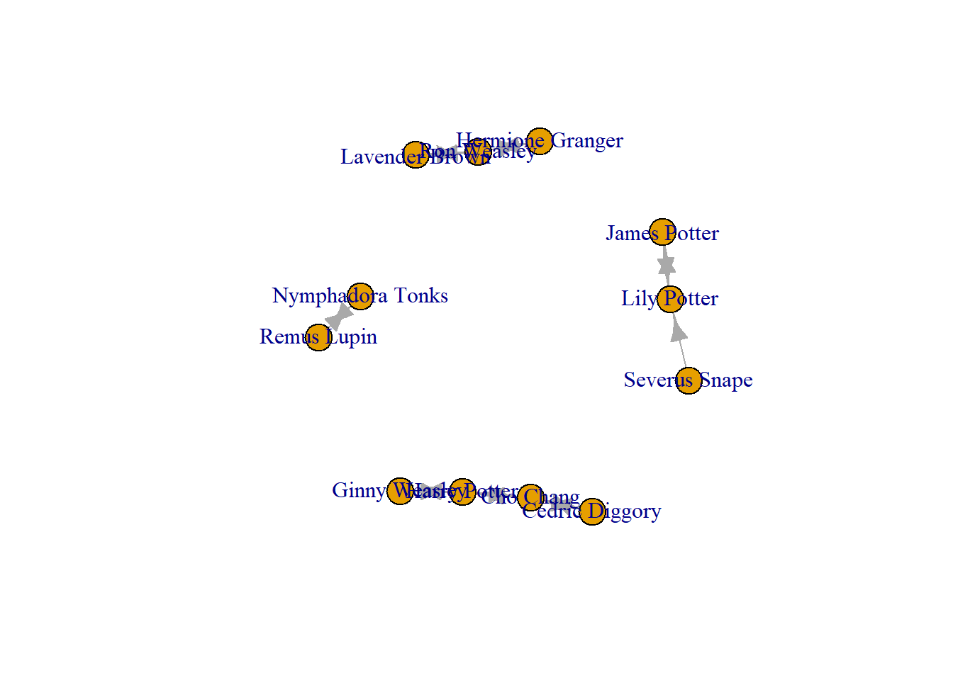
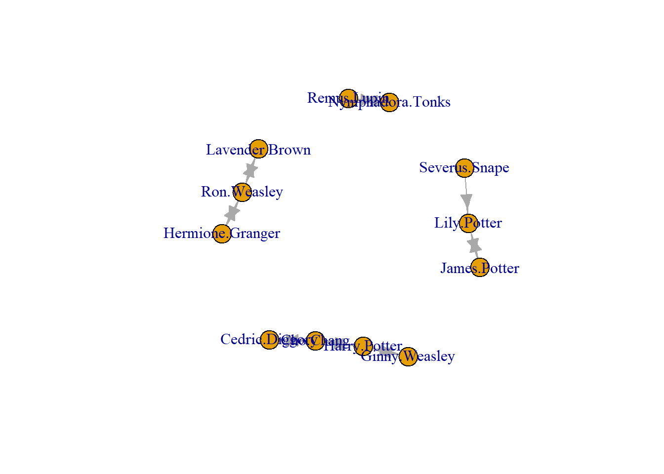
Finally, you can use the plot() function to visualise the network. I plot one, then the other. They reflect the same data but stored and brought into RStudio in different ways.
plot(g1)
plot(g2)
Summary
When working with network data, you need to be mindful of how it is stored and learn the ways to wrangle it from a dataset into a network object ready for further clearning or analysis. In this chapter you have learned three things:
How network data are stored (an edge list or adjacency matrix)
How to bring network data into RStudio and understand it